
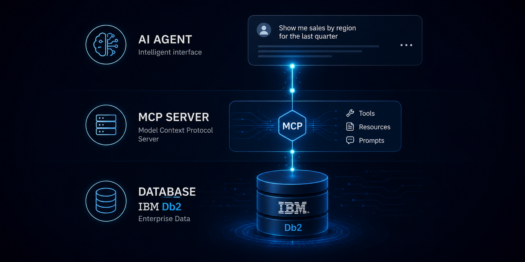
Descubrimiento de esquema, generación de SQL y EXPLAIN con Claude Code y Db2 12.1
Un tutorial completo utilizando una sesión de Claude Code que entiende preguntas en lenguaje natural sobre una base de datos Db2, genera y ejecuta SQL, y explica los planes de acceso a las consultas en términos simples.
Qué vamos a construir
Un servidor MCP que conecta Claude Code directamente a IBM Db2 LUW 12.1 utilizando el driver Python nativo ibm_db. Sin intermediario REST, sin contenedores adicionales. El servidor expone ocho herramientas y un recurso:
| Herramienta | Función |
|---|---|
list_schemas() | Descubrir esquemas dentro de la base de datos conectada |
list_tables(schema) | Tablas de un esquema con estadísticas |
describe_table(schema, table) | Definiciones de columnas, tipos, nullability |
list_indexes(schema, table) | Índices con cluster ratio y columnas clave |
sample_rows(schema, table) | Previsualizar hasta 20 filas |
execute_query(sql) | Ejecutar cualquier SELECT — el motor SQL en lenguaje natural |
explain_query(sql) | EXPLAIN + interpretación en lenguaje simple del plan de acceso |
search_columns(name) | Encontrar todas las tablas que contienen una columna por nombre |
table_dependencies(schema, table) | Objetos que referencian una tabla |
Arquitectura
Claude Code  (lenguaje natural)
      |
      |  JSON-RPC sobre stdio
      v
server.py  (Servidor MCP)
      |
      |  TCP 50000  (ibm_db / clidriver — conexión directa)
      v
IBM Db2 LUW 12.1 Community Edition  (Docker, puerto 50000)
El paquete Python ibm_db incluye el IBM CLI driver y gestiona la conexión. No se necesita ninguna instalación separada del cliente Db2.
Requisitos previos
- Una máquina con Linux
- Docker y Docker Compose
- Python 3.10 o superior
- Claude Code
Parte 1: Entorno Docker
Crear el directorio de trabajo y entrar en él antes de crear el fichero docker-compose.yml:
mkdir db2-mcp-tutorial
cd db2-mcp-tutorial
1.1 docker-compose.yml
La configuración es bastante sencilla. Solo un contenedor ejecutando la instancia Db2.
Crear el fichero directamente desde la shell:
cat > docker-compose.yml <<'EOF'
services:
  db2:
    image: icr.io/db2_community/db2:latest
    privileged: true
    environment:
      LICENSE: accept
      DB2INST1_PASSWORD: passw0rd
    ports:
      - "50000:50000"
    volumes:
      - db2_data:/database
    healthcheck:
      test: ["CMD", "su", "-", "db2inst1", "-c", "db2 list db directory"]
      interval: 30s
      timeout: 10s
      retries: 15
      start_period: 600s

volumes:
  db2_data:
EOF
1.2 Iniciar el contenedor
Ejecutar para arrancar el contenedor Db2.
docker compose up -dEl primer arranque realiza la configuración completa de la instancia y la base de datos Db2. Puede tardar entre 3 y 5 minutos.
Esperar un momento y verificar el estado del contenedor:
docker psSi todavía está iniciando, esperar unos 30 segundos y comprobar de nuevo:
sleep 30
docker ps
No continuar al paso siguiente hasta que el contenedor esté en estado healthy.
1.3 Crear los objetos de ejemplo SAMPLE
Ejecutar db2sampl solo después de que el contenedor esté en estado healthy:
docker compose exec db2 su - db2inst1 -c "db2sampl -sql -force"
# Tarda unos 60 segundos
Verificar que la base de datos y los objetos de esquema están presentes:
docker compose exec db2 su - db2inst1 -c \
  "db2 connect to SAMPLE && db2 'select count(*) as employee_count from employee' && db2 connect reset"
# Esperado: 42
Crear las tablas EXPLAIN en el esquema:
docker compose exec db2 su - db2inst1 -c \
  "db2 connect to SAMPLE && db2 -tf /database/config/db2inst1/sqllib/misc/EXPLAIN.DDL && db2 connect reset"
Parte 2: Estructura del Proyecto y Dependencias
El proyecto tiene esta estructura.
db2-mcp-tutorial/
|- docker-compose.yml
|- server.py
|- pyproject.toml
`- .env
Crear el fichero pyproject.toml directamente desde la shell:
cat > pyproject.toml <<'EOF'
[project]
name = "db2-schema-mcp"
version = "0.1.0"
requires-python = ">=3.10"
dependencies = [
    "mcp[cli]>=1.25",
    "ibm-db>=3.2.0",
    "python-dotenv>=1.0",
]
EOF
Crear el entorno Python local e instalar las dependencias del proyecto:
uv venvcrea un entorno virtual aislado en.venvuv pip install -e .instala el paquete en modo editable y descarga las dependencias declaradas enpyproject.toml
uv venv && uv pip install -e .ibm_db descarga e instala el IBM CLI driver automáticamente. No se requiere ninguna instalación separada del cliente Db2.
Crear el fichero de entorno:
cat > .env <<'EOF'
DB2_HOST=localhost
DB2_PORT=50000
DB2_DBNAME=SAMPLE
DB2_USER=db2inst1
DB2_PASSWORD=passw0rd
EOF
Parte 3: El Servidor MCP (server.py)
Un servidor MCP es un pequeño proceso local que expone capacidades a un cliente de IA de forma estructurada. En lugar de dejar que el modelo invente cómo llegar a Db2, el servidor MCP le proporciona herramientas explícitas como list_tables, describe_table, execute_query y explain_query.
En la práctica, esto significa que el servidor MCP proporciona dos cosas:
- Un puente controlado entre Claude Code y la base de datos Db2
- Una superficie de herramientas definida que el modelo puede invocar de forma segura y predecible
Para este artículo, server.py es ese puente. Recibe llamadas de herramientas de Claude Code vía MCP, abre una conexión ibm_db directa a Db2, ejecuta la operación de metadatos o SQL solicitada, y devuelve el resultado en un formato que el agente puede interpretar.
Para crear el fichero server.py, abrir una sesión vi:
vi server.pyY pegar este contenido en el fichero:
"""
MCP Server — Db2 Schema Explorer
Explores tables, columns, indexes and sample data from an IBM Db2 database.
Connects directly via ibm_db driver (no REST Service required).
Compatible with Db2 LUW 12.1 Community Edition running in Docker.
"""
import os
import threading
import ibm_db
from dotenv import load_dotenv
from mcp.server.fastmcp import FastMCP
load_dotenv()
# ── Configuration ─────────────────────────────────────────────────────────────
DB2_HOST = os.getenv("DB2_HOST", "localhost")
DB2_PORT = os.getenv("DB2_PORT", "50000")
DB2_DBNAME = os.getenv("DB2_DBNAME", "SAMPLE")
DB2_USER = os.getenv("DB2_USER", "db2inst1")
DB2_PASS = os.getenv("DB2_PASSWORD", "passw0rd")
_DSN = (
f"DATABASE={DB2_DBNAME};"
f"HOSTNAME={DB2_HOST};"
f"PORT={DB2_PORT};"
f"PROTOCOL=TCPIP;"
f"UID={DB2_USER};"
f"PWD={DB2_PASS};"
"CONNECTTIMEOUT=30;"
"QUERYTIMEOUT=120;"
)
# ── Connection management ─────────────────────────────────────────────────────
# ibm_db is a synchronous C extension — not thread-safe per connection.
# A global lock serialises all queries. For high-concurrency production use,
# create a new connection per request instead.
_conn_lock = threading.Lock()
_conn: object = None
def _get_conn():
"""Return the active Db2 connection, reconnecting automatically if needed."""
global _conn
try:
if _conn is not None:
ibm_db.active(_conn) # raises if connection is dead
return _conn
except Exception:
_conn = None
_conn = ibm_db.connect(_DSN, "", "")
return _conn
def run_sql(query: str) -> list[dict]:
"""
Execute a SELECT statement and return the result set as a list of dicts.
Thread-safe via global connection lock.
"""
with _conn_lock:
conn = _get_conn()
stmt = ibm_db.exec_immediate(conn, query)
rows: list[dict] = []
row = ibm_db.fetch_assoc(stmt)
while row:
rows.append(dict(row))
row = ibm_db.fetch_assoc(stmt)
ibm_db.free_result(stmt)
return rows
def run_admin_cmd(command: str) -> list[dict]:
"""
Execute an administrative Db2 CLP command via SYSPROC.ADMIN_CMD.
Returns the result set as a list of dicts.
ADMIN_CMD runs commands like LIST DATABASE DIRECTORY, RUNSTATS, etc.
as a stored procedure — no shell access or docker exec required.
"""
with _conn_lock:
conn = _get_conn()
stmt = ibm_db.exec_immediate(
conn, f"CALL SYSPROC.ADMIN_CMD(\'{command}\')"
)
rows: list[dict] = []
row = ibm_db.fetch_assoc(stmt)
while row:
rows.append(dict(row))
row = ibm_db.fetch_assoc(stmt)
ibm_db.free_result(stmt)
return rows
# ── MCP Server ────────────────────────────────────────────────────────────────
mcp = FastMCP(
"db2-schema-explorer",
instructions=(
"You are a Db2 database assistant with tools to inspect an IBM Db2 LUW database.\n\n"
"CRITICAL — DATABASE vs SCHEMA:\n"
"In Db2, the database name (e.g. SAMPLE) is the connection target — it is NOT a schema. "
"Schemas are namespaces INSIDE the database (e.g. DB2INST1, SYSCAT, SYSTOOLS). "
"Never use the database name as a schema parameter.\n\n"
"WORKFLOW:\n"
"0. When the user asks what databases exist on the server, call list_databases().\n"
"1. When the user asks about tables 'in the database' or mentions the database name "
"(e.g. SAMPLE), ALWAYS call list_schemas() first to discover which schemas actually "
"exist — do not assume the database name is a schema.\n"
"2. Then call list_tables(schema) for each schema of interest.\n"
"3. Never guess or assume a schema name. "
"The instance owner schema is typically DB2INST1, not the database name.\n\n"
"TOOL SUMMARY:\n"
"- list_databases() list all databases in the Db2 instance\n"
"- list_schemas() discover all schemas in the database\n"
"- list_tables(schema) tables in a specific schema\n"
"- describe_table(schema,table) column definitions\n"
"- list_indexes(schema,table) index definitions\n"
"- sample_rows(schema,table) preview a few rows (max 20, no filtering)\n"
"- execute_query(sql) run any SELECT — USE THIS for filtering, "
"aggregation, subqueries, joins, ranking, or any analytical question\n"
"- explain_query(sql) explain the access plan for a SELECT and "
"interpret index usage, joins, sorts and cost estimates\n"
"- search_columns(name) find tables that have a column by name\n"
"- table_dependencies(schema,table) objects that depend on a table\n\n"
"WHEN TO USE execute_query:\n"
"Whenever the user asks a question that requires SQL logic — averages, totals, "
"comparisons, filters, GROUP BY, subqueries — generate the correct SQL and call "
"execute_query(sql). Never approximate by sampling rows and calculating manually. "
"Always use fully qualified table names (SCHEMA.TABLE) in the SQL.\n\n"
"Always use uppercase for all schema and table names."
),
)
@mcp.tool()
def list_databases() -> str:
"""
List all databases registered in the Db2 instance directory.
Uses SYSPROC.ADMIN_CMD to run the Db2 CLP command
LIST DATABASE DIRECTORY, which shows every database catalogued
on this instance: name, alias, type (local/remote), and path.
Call this first when the user wants to know what databases are
available on the server, or before connecting to a specific database.
"""
try:
rows = run_admin_cmd("LIST DATABASE DIRECTORY")
except Exception as exc:
return f"Failed to list databases: {exc}"
if not rows:
return "No databases found in the instance directory."
lines = [f"**Databases in instance directory** ({len(rows)} found)\n"]
for r in rows:
alias = r.get("DATABASE_ALIAS", r.get("DB_ALIAS", "?"))
name = r.get("DATABASE_NAME", r.get("DB_NAME", alias))
db_type = r.get("DATABASE_TYPE", r.get("TYPE", "?"))
path = r.get("DATABASE_DIRECTORY", r.get("DIRECTORY", ""))
comment = r.get("COMMENT", "")
lines.append(f"### `{alias}`")
if name != alias:
lines.append(f"- Name : `{name}`")
lines.append(f"- Type : {db_type}")
if path:
lines.append(f"- Directory : `{path}`")
if comment:
lines.append(f"- Comment : {comment}")
return "\n".join(lines)
@mcp.tool()
def list_schemas() -> str:
"""
List all user-defined schemas in the database.
Returns schema name, owner, and creation timestamp.
All Db2 system schemas are excluded (SYS*, SYSIBM, NULLID, SQLJ,
ERRORSCHEMA, SYSTOOLS, DB2GSE, ASMA, SYSPROC).
Call this first whenever the user asks about tables or objects in the
database — do not assume the database name is a schema.
"""
rows = run_sql("""
SELECT SCHEMANAME, OWNER, CREATE_TIME
FROM SYSCAT.SCHEMATA
WHERE SCHEMANAME NOT LIKE 'SYS%'
AND SCHEMANAME NOT IN (
'NULLID', 'SQLJ', 'ERRORSCHEMA',
'SYSTOOLS', 'DB2GSE', 'ASMA', 'SYSPROC'
)
ORDER BY SCHEMANAME
""")
if not rows:
return "No user-defined schemas found."
lines = [f"**Available schemas** ({len(rows)} found)\n"]
for r in rows:
created = str(r.get("CREATE_TIME", ""))[:10]
lines.append(
f"- `{r['SCHEMANAME']}` "
f"(owner: {r.get('OWNER', '?')}, created: {created})"
)
return "\n".join(lines)
@mcp.tool()
def list_tables(schema: str) -> str:
"""
List all tables in a given schema with basic statistics.
Parameters:
schema — schema name (e.g. SAMPLE, DB2INST1). Case-insensitive.
Returns table name, estimated row count (CARD), page count, and last
access date. CARD = -1 means statistics have never been collected
(run RUNSTATS to update).
"""
schema = schema.upper()
rows = run_sql(f"""
SELECT TABNAME, TYPE, CARD, NPAGES, LASTUSED
FROM SYSCAT.TABLES
WHERE TABSCHEMA = '{schema}'
AND TYPE = 'T'
ORDER BY TABNAME
""")
if not rows:
return f"No tables found in schema `{schema}`."
lines = [
f"**Tables in `{schema}`** ({len(rows)} found)\n",
"| Table | Rows (CARD) | Pages | Last used |",
"|-------|-------------|-------|-----------|",
]
for r in rows:
card = r.get("CARD", "?")
npages = r.get("NPAGES", "?")
last_used = str(r.get("LASTUSED", "—"))[:10]
card_flag = " ⚠" if card == -1 else ""
lines.append(
f"| `{r['TABNAME']}` | {card}{card_flag} | {npages} | {last_used} |"
)
if any(r.get("CARD") == -1 for r in rows):
lines.append(
"\n⚠ Tables with CARD = -1 have no statistics. "
"Run `RUNSTATS ON TABLE <schema>.<table>` to collect them."
)
return "\n".join(lines)
@mcp.tool()
def describe_table(schema: str, table: str) -> str:
"""
Describe the column structure of a table.
Parameters:
schema — schema name (e.g. SAMPLE)
table — table name (e.g. EMPLOYEE)
Returns each column's name, data type (with length/scale), nullability,
default value, identity flag, and any column remarks.
"""
schema = schema.upper()
table = table.upper()
rows = run_sql(f"""
SELECT COLNO, COLNAME, TYPENAME, LENGTH, SCALE,
NULLS, DEFAULT, IDENTITY, GENERATED, REMARKS
FROM SYSCAT.COLUMNS
WHERE TABSCHEMA = '{schema}'
AND TABNAME = '{table}'
ORDER BY COLNO
""")
if not rows:
return f"Table `{schema}.{table}` not found or has no columns."
lines = [
f"**`{schema}.{table}`** — {len(rows)} column(s)\n",
"| # | Column | Type | Nullable | Identity | Default | Remarks |",
"|---|--------|------|----------|----------|---------|---------|",
]
for r in rows:
length = f"({r['LENGTH']})" if r.get("LENGTH") else ""
scale = f",{r['SCALE']}" if r.get("SCALE") else ""
col_type = f"{r['TYPENAME']}{length}{scale}"
nullable = "Yes" if r.get("NULLS") == "Y" else "**No**"
identity = "Yes" if r.get("IDENTITY") == "Y" else "—"
default = r.get("DEFAULT") or "—"
remarks = r.get("REMARKS") or "—"
lines.append(
f"| {r['COLNO']} | `{r['COLNAME']}` | `{col_type}` "
f"| {nullable} | {identity} | {default} | {remarks} |"
)
return "\n".join(lines)
@mcp.tool()
def list_indexes(schema: str, table: str) -> str:
"""
List all indexes defined on a table.
Parameters:
schema — schema name
table — table name
Returns index name, type (REG/CLUS/BLOK), uniqueness rule (PK/Unique/Non-unique),
number of leaf pages, tree levels, cluster ratio, and indexed columns
(including ASC/DESC ordering).
"""
schema = schema.upper()
table = table.upper()
rows = run_sql(f"""
SELECT
I.INDNAME,
I.UNIQUERULE,
I.INDEXTYPE,
I.NLEAF,
I.NLEVELS,
I.CLUSTERRATIO,
LISTAGG(
K.COLNAME || CASE K.COLORDER WHEN 'D' THEN ' DESC' ELSE '' END,
', '
) WITHIN GROUP (ORDER BY K.COLSEQ) AS COLUMNS
FROM SYSCAT.INDEXES I
JOIN SYSCAT.INDEXCOLUSE K
ON I.INDSCHEMA = K.INDSCHEMA
AND I.INDNAME = K.INDNAME
WHERE I.TABSCHEMA = '{schema}'
AND I.TABNAME = '{table}'
GROUP BY
I.INDNAME, I.UNIQUERULE, I.INDEXTYPE,
I.NLEAF, I.NLEVELS, I.CLUSTERRATIO
ORDER BY I.INDNAME
""")
if not rows:
return f"No indexes found on `{schema}.{table}`."
unique_map = {"U": "✅ Unique", "P": "✅ PK", "D": "No"}
lines = [
f"**Indexes on `{schema}.{table}`** ({len(rows)} found)\n",
"| Index | Type | Unique | Leaves | Levels | Cluster% | Columns |",
"|-------|------|--------|--------|--------|----------|---------|",
]
for r in rows:
cr = r.get("CLUSTERRATIO", -1)
cluster = f"{cr}%" if cr is not None and cr >= 0 else "?"
lines.append(
f"| `{r['INDNAME']}` "
f"| {r.get('INDEXTYPE', '?')} "
f"| {unique_map.get(r.get('UNIQUERULE', 'D'), '?')} "
f"| {r.get('NLEAF', '?')} "
f"| {r.get('NLEVELS', '?')} "
f"| {cluster} "
f"| `{r.get('COLUMNS', '?')}` |"
)
return "\n".join(lines)
@mcp.tool()
def sample_rows(schema: str, table: str, limit: int = 5) -> str:
"""
Preview the first N rows of a table.
Parameters:
schema — schema name
table — table name
limit — number of rows to return, between 1 and 20 (default: 5)
Returns the rows formatted as a Markdown table. Column values are
truncated to 50 characters to keep the output readable.
"""
schema = schema.upper()
table = table.upper()
limit = max(1, min(limit, 20))
rows = run_sql(f"""
SELECT * FROM {schema}.{table}
FETCH FIRST {limit} ROWS ONLY
""")
if not rows:
return f"Table `{schema}.{table}` is empty or does not exist."
headers = list(rows[0].keys())
lines = [
f"**`{schema}.{table}`** — first {len(rows)} row(s)\n",
"| " + " | ".join(headers) + " |",
"| " + " | ".join(["---"] * len(headers)) + " |",
]
for r in rows:
cells = [str(r.get(h, ""))[:50] for h in headers]
lines.append("| " + " | ".join(cells) + " |")
return "\n".join(lines)
@mcp.tool()
def execute_query(sql: str, max_rows: int = 100) -> str:
"""
Execute a read-only SQL SELECT statement and return the full result set.
Use this tool whenever the user asks a question that requires filtering,
aggregation, joining, subqueries, or any logic beyond a simple row preview.
Examples: averages, totals, rankings, comparisons, EXISTS, GROUP BY, HAVING.
Parameters:
sql — a valid Db2 SQL SELECT statement.
Must be a SELECT — INSERT, UPDATE, DELETE and DDL are rejected.
Schema and table names must be fully qualified (e.g. DB2INST1.EMPLOYEE).
max_rows — maximum number of rows to return (default: 100, maximum: 500).
The tool executes the SQL exactly as provided. Generate correct, complete SQL
before calling — do not call with placeholder or incomplete statements.
Example queries:
SELECT * FROM DB2INST1.EMPLOYEE
WHERE SALARY > (SELECT AVG(SALARY) FROM DB2INST1.EMPLOYEE)
ORDER BY SALARY DESC
SELECT WORKDEPT, COUNT(*) AS HEADCOUNT, AVG(SALARY) AS AVG_SALARY
FROM DB2INST1.EMPLOYEE
GROUP BY WORKDEPT
ORDER BY AVG_SALARY DESC
"""
# Safety: only allow SELECT statements
sql_stripped = sql.strip().upper()
if not sql_stripped.startswith("SELECT") and \
not sql_stripped.startswith("WITH"):
return (
"Error: only SELECT (or WITH ... SELECT) statements are allowed. "
"INSERT, UPDATE, DELETE and DDL are not permitted."
)
max_rows = max(1, min(max_rows, 500))
# Append FETCH FIRST if not already present
if "FETCH FIRST" not in sql_stripped:
sql = f"{sql.rstrip().rstrip(';')} FETCH FIRST {max_rows} ROWS ONLY"
try:
rows = run_sql(sql)
except Exception as exc:
return f"Query failed:\n```\n{exc}\n```"
if not rows:
return "Query executed successfully — no rows returned."
headers = list(rows[0].keys())
lines = [
f"**Query result** — {len(rows)} row(s)\n",
"| " + " | ".join(headers) + " |",
"| " + " | ".join(["---"] * len(headers)) + " |",
]
for r in rows:
cells = [str(r.get(h, ""))[:60] for h in headers]
lines.append("| " + " | ".join(cells) + " |")
if len(rows) == max_rows:
lines.append(
f"\n*Result limited to {max_rows} rows. "
"Pass a higher max_rows value to retrieve more.*"
)
return "\n".join(lines)
@mcp.tool()
def search_columns(column_name: str) -> str:
"""
Find all tables that contain a column matching the given name pattern.
Parameters:
column_name — full or partial column name to search for.
The search is case-insensitive and uses SQL LIKE
with wildcards on both sides (e.g. 'DATE' matches
ORDER_DATE, HIRE_DATE, etc.).
Returns schema, table, column name, data type, and nullability.
Results are limited to 50 rows and exclude system schemas.
"""
pattern = column_name.upper()
rows = run_sql(f"""
SELECT TABSCHEMA, TABNAME, COLNAME, TYPENAME, NULLS
FROM SYSCAT.COLUMNS
WHERE COLNAME LIKE '%{pattern}%'
AND TABSCHEMA NOT LIKE 'SYS%'
ORDER BY TABSCHEMA, TABNAME, COLNAME
FETCH FIRST 50 ROWS ONLY
""")
if not rows:
return f"No columns matching `%{pattern}%` found."
lines = [
f"**Columns matching `%{pattern}%`** ({len(rows)} found)\n",
"| Schema | Table | Column | Type | Nullable |",
"|--------|-------|--------|------|----------|",
]
for r in rows:
nullable = "Yes" if r.get("NULLS") == "Y" else "No"
lines.append(
f"| `{r['TABSCHEMA']}` | `{r['TABNAME']}` "
f"| `{r['COLNAME']}` | {r['TYPENAME']} | {nullable} |"
)
return "\n".join(lines)
@mcp.tool()
def table_dependencies(schema: str, table: str) -> str:
"""
List objects that depend on a given table: views, triggers, packages,
and stored procedures that reference it.
Parameters:
schema — schema name
table — table name
Useful before performing ALTER TABLE or DROP TABLE to understand
the impact on dependent objects.
"""
schema = schema.upper()
table = table.upper()
rows = run_sql(f"""
SELECT DNAME AS OBJECT_NAME, DTYPE AS OBJECT_TYPE, TABSCHEMA
FROM SYSCAT.PACKAGEDEP
WHERE BSCHEMA = '{schema}'
AND BNAME = '{table}'
AND BTYPE = 'T'
UNION ALL
SELECT VIEWNAME, 'V', VIEWSCHEMA
FROM SYSCAT.VIEWDEP
WHERE BSCHEMA = '{schema}'
AND BNAME = '{table}'
ORDER BY OBJECT_TYPE, OBJECT_NAME
""")
if not rows:
return (
f"No dependencies found for `{schema}.{table}`.\n\n"
"This does not guarantee the table is unused — "
"application-level references are not tracked here."
)
type_map = {
"V": "View",
"R": "Stored Procedure",
"F": "Function",
"T": "Trigger",
"P": "Package",
}
lines = [
f"**Dependencies of `{schema}.{table}`** ({len(rows)} found)\n",
"| Type | Object |",
"|------|--------|",
]
for r in rows:
obj_type = type_map.get(r.get("OBJECT_TYPE", "?"), r.get("OBJECT_TYPE", "?"))
lines.append(f"| {obj_type} | `{r.get('OBJECT_NAME', '?')}` |")
lines.append(
"\n⚠ Any structural change to this table may invalidate the objects listed above."
)
return "\n".join(lines)
# ── EXPLAIN ───────────────────────────────────────────────────────────────────
def _to_float(value) -> float:
"""Parse a cost value returned by Db2 DECIMAL(), tolerating locale-specific
decimal separators (e.g. '13,64' on European-locale servers)."""
if value is None:
return 0.0
s = str(value).strip()
if ',' in s and '.' in s:
if s.rfind(',') > s.rfind('.'):
s = s.replace('.', '').replace(',', '.')
else:
s = s.replace(',', '')
else:
s = s.replace(',', '.')
return float(s) if s else 0.0
@mcp.tool()
def explain_query(sql: str) -> str:
"""
Explain the access plan for a SQL SELECT statement and interpret it
in plain English.
Parameters:
sql — a valid Db2 SELECT statement to explain.
Must not contain EXPLAIN PLAN FOR — provide only the SELECT.
What this tool does:
1. Runs EXPLAIN PLAN FOR <sql> to populate the explain tables.
2. Reads EXPLAIN_OPERATOR, EXPLAIN_PREDICATE and EXPLAIN_ARGUMENT
to extract the full access plan.
3. Returns a formatted report with an operator table, predicate
details, and a plain-English interpretation of the access path.
Operator types and their meaning:
RETURN — final output node (root of the tree)
TBSCAN — Table Scan: reads every row in the table (expensive for large tables)
IXSCAN — Index Scan: uses an index to find rows (efficient)
FETCH — retrieves full rows after an index lookup
NLJOIN — Nested Loop Join: for each row in outer, scans inner (good for small sets)
HSJOIN — Hash Join: builds hash table, good for large unsorted sets
MSJOIN — Merge Scan Join: both inputs sorted, good for sorted data
SORT — sorts the data (may spill to disk if SORTHEAP is small)
GRPBY — Group By / aggregation
FILTER — applies a predicate filter
TEMP — materialises intermediate results to a temp table
"""
try:
with _conn_lock:
conn = _get_conn()
ibm_db.exec_immediate(conn, f"EXPLAIN PLAN FOR {sql}")
except Exception as exc:
return f"EXPLAIN failed: {exc}"
# Read operator tree (most recent explain for this session)
operators = run_sql("""
SELECT
E.OPERATOR_ID,
E.OPERATOR_TYPE,
S.OBJECT_SCHEMA,
S.OBJECT_NAME,
DECIMAL(E.TOTAL_COST, 15, 2) AS TOTAL_COST,
DECIMAL(E.IO_COST, 15, 2) AS IO_COST,
DECIMAL(E.CPU_COST, 15, 2) AS CPU_COST,
E.FIRST_ROW_COST,
C.OUTPUT_CARD
FROM EXPLAIN_OPERATOR E
LEFT JOIN (
SELECT EXPLAIN_TIME, TARGET_ID,
MIN(OBJECT_SCHEMA) AS OBJECT_SCHEMA,
MIN(OBJECT_NAME) AS OBJECT_NAME
FROM EXPLAIN_STREAM
WHERE SOURCE_TYPE = 'D'
AND OBJECT_NAME IS NOT NULL
GROUP BY EXPLAIN_TIME, TARGET_ID
) S ON E.EXPLAIN_TIME = S.EXPLAIN_TIME
AND E.OPERATOR_ID = S.TARGET_ID
LEFT JOIN (
SELECT EXPLAIN_TIME, SOURCE_ID,
DECIMAL(MIN(STREAM_COUNT), 15, 2) AS OUTPUT_CARD
FROM EXPLAIN_STREAM
WHERE SOURCE_TYPE = 'O'
GROUP BY EXPLAIN_TIME, SOURCE_ID
) C ON E.EXPLAIN_TIME = C.EXPLAIN_TIME
AND E.OPERATOR_ID = C.SOURCE_ID
WHERE E.EXPLAIN_TIME = (
SELECT MAX(EXPLAIN_TIME) FROM EXPLAIN_INSTANCE
)
ORDER BY E.OPERATOR_ID
""")
# Step 4 — read predicates
predicates = run_sql("""
SELECT
P.OPERATOR_ID,
P.HOW_APPLIED,
SUBSTR(P.PREDICATE_TEXT, 1, 120) AS PREDICATE_TEXT
FROM EXPLAIN_PREDICATE P
WHERE P.EXPLAIN_TIME = (
SELECT MAX(EXPLAIN_TIME) FROM EXPLAIN_INSTANCE
)
ORDER BY P.OPERATOR_ID, P.HOW_APPLIED
""")
# Step 5 — read operator arguments (access type, index name, etc.)
arguments = run_sql("""
SELECT
A.OPERATOR_ID,
A.ARGUMENT_TYPE,
SUBSTR(A.ARGUMENT_VALUE, 1, 80) AS ARGUMENT_VALUE
FROM EXPLAIN_ARGUMENT A
WHERE A.EXPLAIN_TIME = (
SELECT MAX(EXPLAIN_TIME) FROM EXPLAIN_INSTANCE
)
AND A.ARGUMENT_TYPE IN (
'SCANDIR','PREFETCH','ROWLOCK','TABLOCK',
'UNIQUE','OUTERJOIN','JOIN TYPE','ACCESSTYPE'
)
ORDER BY A.OPERATOR_ID, A.ARGUMENT_TYPE
""")
if not operators:
return "No explain plan was generated. Check that the SQL is valid."
# Build predicate map: operator_id → list of (how_applied, text)
pred_map: dict[int, list] = {}
for p in predicates:
oid = int(p.get("OPERATOR_ID", 0))
pred_map.setdefault(oid, []).append(
(p.get("HOW_APPLIED", "?"), p.get("PREDICATE_TEXT", ""))
)
# Build argument map: operator_id → dict of argument_type → value
arg_map: dict[int, dict] = {}
for a in arguments:
oid = int(a.get("OPERATOR_ID", 0))
arg_map.setdefault(oid, {})[a.get("ARGUMENT_TYPE", "")] = \
a.get("ARGUMENT_VALUE", "")
# Operator type descriptions
op_desc = {
"RETURN": "Return (final output)",
"TBSCAN": "Table Scan ⚠ (full table read)",
"IXSCAN": "Index Scan ✅",
"FETCH": "Fetch (row retrieval after index)",
"NLJOIN": "Nested Loop Join",
"HSJOIN": "Hash Join",
"MSJOIN": "Merge Scan Join",
"SORT": "Sort ⚠",
"GRPBY": "Group By / Aggregate",
"FILTER": "Filter",
"TEMP": "Temp Materialisation",
"UNION": "Union",
"EXCEPT": "Except",
"IXAND": "Index AND (multiple indexes combined)",
"RIDSCN": "RID Scan",
}
# Build output
total_cost = sum(
_to_float(r.get("TOTAL_COST"))
for r in operators
if r.get("OPERATOR_TYPE") == "RETURN"
)
lines = [
"**EXPLAIN — Access Plan**\n",
f"**Estimated total cost:** {total_cost:,.2f} timerons\n",
"| Op | Type | Object | Total Cost | IO Cost | Output Rows |",
"|----|------|--------|-----------|---------|-------------|",
]
has_tbscan = False
has_sort = False
has_ixscan = False
for r in operators:
op_id = int(r.get("OPERATOR_ID", 0))
op_type = r.get("OPERATOR_TYPE", "?")
obj = ""
if r.get("OBJECT_NAME"):
obj = f"`{r.get('OBJECT_SCHEMA','')}.{r['OBJECT_NAME']}`"
cost = r.get("TOTAL_COST", "?")
io_cost = r.get("IO_COST", "?")
card = r.get("OUTPUT_CARD", "?")
label = op_desc.get(op_type, op_type)
if op_type == "TBSCAN": has_tbscan = True
if op_type == "SORT": has_sort = True
if op_type == "IXSCAN": has_ixscan = True
args = arg_map.get(op_id, {})
access = args.get("ACCESSTYPE", "")
if access:
label += f" [{access}]"
lines.append(
f"| {op_id} | {label} | {obj} "
f"| {cost} | {io_cost} | {card} |"
)
for how, text in pred_map.get(op_id, []):
pred_icon = "✅" if how in ("SARG", "RANGE", "MATCH") else "⚠"
lines.append(
f"| | ↳ Predicate `{how}` {pred_icon} "
f"| `{text}` | | | |"
)
# ── Plain-English interpretation ─────────────────────────────────────────
lines.append("\n---\n**Interpretation:**\n")
if has_ixscan and not has_tbscan:
lines.append(
"✅ **Index usage:** the query uses index scans — "
"the optimizer found suitable indexes for the predicates."
)
elif has_tbscan and not has_ixscan:
lines.append(
"⚠ **Table scan detected:** the optimizer is reading the entire table. "
"This is acceptable for small tables but expensive for large ones. "
"Consider creating an index on the columns used in WHERE or JOIN conditions."
)
elif has_tbscan and has_ixscan:
lines.append(
"⚠ **Mixed access:** some tables use indexes, others use full scans. "
"Review the TBSCAN operators — those tables may benefit from indexes."
)
if has_sort:
lines.append(
"⚠ **Sort operation present:** the query requires sorting. "
"If this is for an ORDER BY or GROUP BY, consider an index "
"that matches the sort order to eliminate the sort operator."
)
if total_cost > 100000:
lines.append(
f"⚠ **High estimated cost ({total_cost:,.0f} timerons):** "
"this query may be expensive. Review table scans and sort operations. "
"Ensure RUNSTATS has been run recently so the optimizer has accurate statistics."
)
elif total_cost < 100:
lines.append(
f"✅ **Low estimated cost ({total_cost:,.0f} timerons):** "
"the query is expected to be fast."
)
lines.append(
"\n*Note: costs are estimates based on catalog statistics. "
"Run `RUNSTATS ON TABLE <schema>.<table> WITH DISTRIBUTION AND INDEXES ALL` "
"if statistics are stale (CARD = -1 or outdated).*"
)
return "\n".join(lines)
# ── Resource — schema overview ────────────────────────────────────────────────
@mcp.resource("db2://schema/{schema}/overview")
def schema_overview(schema: str) -> str:
"""
High-level summary of a schema: table count, total rows, and total pages.
Loaded as background context before answering schema-level questions.
"""
schema = schema.upper()
rows = run_sql(f"""
SELECT
COUNT(*) AS NUM_TABLES,
SUM(CARD) AS TOTAL_ROWS,
SUM(NPAGES) AS TOTAL_PAGES
FROM SYSCAT.TABLES
WHERE TABSCHEMA = '{schema}'
AND TYPE = 'T'
""")
if not rows or not rows[0].get("NUM_TABLES"):
return f"Schema `{schema}` not found or empty."
r = rows[0]
return (
f"Schema: {schema}\n"
f"Tables: {r.get('NUM_TABLES', '?')}\n"
f"Total rows (estimated): {r.get('TOTAL_ROWS', '?')}\n"
f"Total pages: {r.get('TOTAL_PAGES', '?')}\n"
)
# ── Entry point ───────────────────────────────────────────────────────────────
if __name__ == "__main__":
print(f"Connecting to Db2: {DB2_HOST}:{DB2_PORT}/{DB2_DBNAME} as {DB2_USER}")
try:
test = run_sql("SELECT 1 AS OK FROM SYSIBM.SYSDUMMY1")
print(f"Connection OK — server ready.")
except Exception as exc:
print(f"Connection FAILED: {exc}")
raise
mcp.run(transport="stdio")El fichero completo está ahora creado. Las subsecciones siguientes explican solo las partes más importantes de server.py sección por sección.
3.1 Gestión de la conexión
Como ibm_db es una extensión C síncrona, no soporta async/await de Python. Todas las funciones de herramientas se definen con def (no async def). Un threading.Lock() global serializa las consultas porque ibm_db no es thread-safe por conexión.
_DSN = (
    f"DATABASE={DB2_DBNAME};"
    f"HOSTNAME={DB2_HOST};"
    f"PORT={DB2_PORT};"
    f"PROTOCOL=TCPIP;"
    f"UID={DB2_USER};"
    f"PWD={DB2_PASS};"
    "CONNECTTIMEOUT=30;"
    "QUERYTIMEOUT=120;"
)

_conn_lock = threading.Lock()
_conn: object = None

def _get_conn():
    global _conn
    try:
        if _conn is not None:
            ibm_db.active(_conn)
            return _conn
    except Exception:
        _conn = None
    _conn = ibm_db.connect(_DSN, "", "")
    return _conn
3.2 Dos funciones auxiliares de ejecución
def run_sql(query: str) -> list[dict]:
    with _conn_lock:
        conn = _get_conn()
        stmt = ibm_db.exec_immediate(conn, query)
        rows = []
        row = ibm_db.fetch_assoc(stmt)
        while row:
            rows.append(dict(row))
            row = ibm_db.fetch_assoc(stmt)
        ibm_db.free_result(stmt)
        return rows

def run_admin_cmd(command: str) -> list[dict]:
    with _conn_lock:
        conn = _get_conn()
        safe_command = command.replace("'", "''")
        stmt = ibm_db.exec_immediate(conn, f"CALL SYSPROC.ADMIN_CMD('{safe_command}')")
        rows = []
        row = ibm_db.fetch_assoc(stmt)
        while row:
            rows.append(dict(row))
            row = ibm_db.fetch_assoc(stmt)
        ibm_db.free_result(stmt)
        return rows
run_admin_cmd usa SYSPROC.ADMIN_CMD, el stored procedure de IBM para comandos CLP.
3.3 Instrucciones del agente
El parámetro instructions de FastMCP es el texto que Claude lee al arrancar. Define cómo debe comportarse el agente:
mcp = FastMCP(
    "db2-schema-explorer",
    instructions=(
        "You are a Db2 database assistant with tools to inspect an IBM Db2 LUW database.\n\n"

        "CRITICAL — DATABASE vs SCHEMA:\n"
        "In Db2, the database name (e.g. SAMPLE) is the connection target — it is NOT a schema. "
        "Schemas are namespaces INSIDE the database (e.g. DB2INST1, SYSCAT, SYSTOOLS). "
        "Never use the database name as a schema parameter.\n\n"

        "WORKFLOW:\n"
        "0. When the user asks what databases exist on the server, call list_databases().\n"
        "1. When the user asks about tables 'in the database' or mentions the database name "
        "(e.g. SAMPLE), ALWAYS call list_schemas() first to discover which schemas actually "
        "exist — do not assume the database name is a schema.\n"
        "2. Then call list_tables(schema) for each schema of interest.\n"
        "3. Never guess or assume a schema name. "
        "The instance owner schema is typically DB2INST1, not the database name.\n\n"

        "TOOL SUMMARY:\n"
        "- list_databases()             list all databases in the Db2 instance\n"
        "- list_schemas()               discover all schemas in the database\n"
        "- list_tables(schema)          tables in a specific schema\n"
        "- describe_table(schema,table) column definitions\n"
        "- list_indexes(schema,table)   index definitions\n"
        "- sample_rows(schema,table)    preview a few rows (max 20, no filtering)\n"
        "- execute_query(sql)           run any SELECT — USE THIS for filtering, "
        "aggregation, subqueries, joins, ranking, or any analytical question\n"
        "- explain_query(sql)           explain the access plan for a SELECT and "
        "interpret index usage, joins, sorts and cost estimates\n"
        "- search_columns(name)         find tables that have a column by name\n"
        "- table_dependencies(schema,table) objects that depend on a table\n\n"

        "WHEN TO USE execute_query:\n"
        "Whenever the user asks a question that requires SQL logic — averages, totals, "
        "comparisons, filters, GROUP BY, subqueries — generate the correct SQL and call "
        "execute_query(sql). Never approximate by sampling rows and calculating manually. "
        "Always use fully qualified table names (SCHEMA.TABLE) in the SQL.\n\n"

        "Always use uppercase for all schema and table names."
    ),
)
3.4 La herramienta execute_query
Esta es la herramienta central para análisis en lenguaje natural. Una vez que Claude ha descubierto el esquema y comprendido la estructura de las tablas, execute_query es la función que ejecuta el SQL generado contra Db2.
Tres decisiones de diseño son importantes aquí:
- Solo acepta instrucciones
SELECTyWITH ... SELECT, por lo que el agente no puede modificar datos - Añade
FETCH FIRST n ROWS ONLYautomáticamente cuando el SQL no incluye ya un límite de filas - Devuelve el resultado como tabla Markdown formateada que Claude Code puede leer y resumir directamente
@mcp.tool()
def execute_query(sql: str, max_rows: int = 100) -> str:
    sql_stripped = sql.strip().upper()
    if not sql_stripped.startswith("SELECT") and not sql_stripped.startswith("WITH"):
        return "Error: only SELECT or WITH ... SELECT statements are allowed."

    max_rows = max(1, min(max_rows, 500))
    if "FETCH FIRST" not in sql_stripped:
        sql = f"{sql.rstrip(';')} FETCH FIRST {max_rows} ROWS ONLY"

    try:
        rows = run_sql(sql)
    except Exception as exc:
        return f"Query failed:\n{exc}"
    return json.dumps(rows, indent=2, default=str)
3.5 La herramienta explain_query
La herramienta emite EXPLAIN PLAN FOR <sql> vía exec_immediate para rellenar las tablas de explain, y luego consulta tres tablas EXPLAIN en secuencia: EXPLAIN_OPERATOR para el árbol de operadores y las estimaciones de coste, EXPLAIN_PREDICATE para las condiciones de predicado en cada nodo, y EXPLAIN_ARGUMENT para los argumentos de los operadores como el tipo de acceso y la dirección de lectura. El resultado es un informe Markdown formateado — tabla de operadores, predicados en línea e interpretación en lenguaje llano del uso de índices, métodos de join, operaciones de ordenación y coste global.
Las tablas EXPLAIN deben ya existir. Se crean en la Parte 1 de este tutorial con el comando db2 -tf EXPLAIN.DDL.
Parte 4: Conectar a Claude Code
Si ya existe una entrada db2-schema más antigua en Claude Code, eliminarla primero:
claude mcp remove db2-schemaLuego añadir el servidor MCP:
claude mcp add db2-schema uv run server.py

claude mcp list
# db2-schema   stdio   uv run server.py

claude
Parte 5: Sesiones de Prueba
En este punto, el servidor MCP está registrado en Claude Code y la base de datos de ejemplo está disponible. Las sesiones siguientes validan el flujo completo: descubrimiento de esquema, generación de SQL, interpretación de resultados y análisis de planes de acceso con EXPLAIN.
Cada sesión proporciona una instrucción para pegar en Claude Code y muestra el tipo de respuesta que se puede esperar del agente.
Sesión 1 — Descubrimiento de Base de Datos y Esquema
Escribir en Claude Code:
What schemas exist inside SAMPLE?Claude (llama a list_schemas()) y devuelve algo como:
The SAMPLE database has 3 schemas:

  ┌──────────┬────────┬─────────────────────┐
  │  Schema  │ Owner  │       Created       │
  ├──────────┼────────┼─────────────────────┤
  │ DB2INST1 │ SYSIBM │ 2026-05-17 19:32:20 │
  ├──────────┼────────┼─────────────────────┤
  │ NULLID   │ SYSIBM │ 2026-05-17 19:31:06 │
  ├──────────┼────────┼─────────────────────┤
  │ SQLJ     │ SYSIBM │ 2026-05-17 19:31:06 │
  └──────────┴────────┴─────────────────────┘

  DB2INST1 is the main user schema where your application tables will live. NULLID and SQLJ are system schemas used internally by Db2. Want me to list
  the tables in DB2INST1?
Escribir en Claude Code:
List the tables in the DB2INST1 schema.Claude (llama a list_tables("DB2INST1")) y devuelve:
The DB2INST1 schema has 15 tables:

  ┌────────────┬───────────┬───────┐
  │   Table    │ Row Count │ Pages │
  ├────────────┼───────────┼───────┤
  │ ACT        │ —         │ —     │
  ├────────────┼───────────┼───────┤
  │ CL_SCHED   │ —         │ —     │
  ├────────────┼───────────┼───────┤
  │ DEPARTMENT │ —         │ —     │
  ├────────────┼───────────┼───────┤
  │ EMPLOYEE   │ —         │ —     │
  ├────────────┼───────────┼───────┤
  │ EMPMDC     │ 10,000    │ 40    │
  ├────────────┼───────────┼───────┤
  │ EMPPROJACT │ —         │ —     │
  ├────────────┼───────────┼───────┤
  │ EMP_PHOTO  │ —         │ —     │
  ├────────────┼───────────┼───────┤
  │ EMP_RESUME │ —         │ —     │
  ├────────────┼───────────┼───────┤
  │ IN_TRAY    │ —         │ —     │
  ├────────────┼───────────┼───────┤
  │ ORG        │ —         │ —     │
  ├────────────┼───────────┼───────┤
  │ PROJACT    │ —         │ —     │
  ├────────────┼───────────┼───────┤
  │ PROJECT    │ —         │ —     │
  ├────────────┼───────────┼───────┤
  │ SALES      │ —         │ —     │
  ├────────────┼───────────┼───────┤
  │ STAFF      │ —         │ —     │
  ├────────────┼───────────┼───────┤
  │ STAFFG     │ —         │ —     │
  └────────────┴───────────┴───────┘

  These are the classic Db2 SAMPLE database tables. Most show -1 for row count (stats not yet collected), except EMPMDC which has 10,000 rows. Would
  you like me to describe any of these tables or run a query?
Sesión 2 — Estructura de Tablas e Índices
Escribir en Claude Code:
Describe the structure of the EMPLOYEE table.Claude (llama a describe_table("DB2INST1", "EMPLOYEE"))
The DB2INST1.EMPLOYEE table has 14 columns:

  ┌─────┬───────────┬──────────────┬────────┬──────────┬─────────────────┐
  │  #  │  Column   │     Type     │ Length │ Nullable │      Notes      │
  ├─────┼───────────┼──────────────┼────────┼──────────┼─────────────────┤
  │ 1   │ EMPNO     │ CHAR         │ 6      │ No       │ Primary key     │
  ├─────┼───────────┼──────────────┼────────┼──────────┼─────────────────┤
  │ 2   │ FIRSTNME  │ VARCHAR      │ 12     │ No       │                 │
  ├─────┼───────────┼──────────────┼────────┼──────────┼─────────────────┤
  │ 3   │ MIDINIT   │ CHAR         │ 1      │ Yes      │ Middle initial  │
  ├─────┼───────────┼──────────────┼────────┼──────────┼─────────────────┤
  │ 4   │ LASTNAME  │ VARCHAR      │ 15     │ No       │                 │
  ├─────┼───────────┼──────────────┼────────┼──────────┼─────────────────┤
  │ 5   │ WORKDEPT  │ CHAR         │ 3      │ Yes      │ FK → DEPARTMENT │
  ├─────┼───────────┼──────────────┼────────┼──────────┼─────────────────┤
  │ 6   │ PHONENO   │ CHAR         │ 4      │ Yes      │                 │
  ├─────┼───────────┼──────────────┼────────┼──────────┼─────────────────┤
  │ 7   │ HIREDATE  │ DATE         │ —      │ Yes      │                 │
  ├─────┼───────────┼──────────────┼────────┼──────────┼─────────────────┤
  │ 8   │ JOB       │ CHAR         │ 8      │ Yes      │                 │
  ├─────┼───────────┼──────────────┼────────┼──────────┼─────────────────┤
  │ 9   │ EDLEVEL   │ SMALLINT     │ —      │ No       │ Education level │
  ├─────┼───────────┼──────────────┼────────┼──────────┼─────────────────┤
  │ 10  │ SEX       │ CHAR         │ 1      │ Yes      │                 │
  ├─────┼───────────┼──────────────┼────────┼──────────┼─────────────────┤
  │ 11  │ BIRTHDATE │ DATE         │ —      │ Yes      │                 │
  ├─────┼───────────┼──────────────┼────────┼──────────┼─────────────────┤
  │ 12  │ SALARY    │ DECIMAL(9,2) │ —      │ Yes      │                 │
  ├─────┼───────────┼──────────────┼────────┼──────────┼─────────────────┤
  │ 13  │ BONUS     │ DECIMAL(9,2) │ —      │ Yes      │                 │
  ├─────┼───────────┼──────────────┼────────┼──────────┼─────────────────┤
  │ 14  │ COMM      │ DECIMAL(9,2) │ —      │ Yes      │ Commission      │
  └─────┴───────────┴──────────────┴────────┴──────────┴─────────────────┘

  EMPNO is the primary key (6-char fixed), WORKDEPT links to the DEPARTMENT table. The three compensation columns — SALARY, BONUS, and COMM — are all
  DECIMAL(9,2). Would you like to sample some rows or run a query against this table?
Escribir en Claude Code:
What indexes does EMPLOYEE have?Claude (llama a list_indexes("DB2INST1", "EMPLOYEE"))
The EMPLOYEE table has 2 indexes:

┌─────────────┬──────────────────────┬───────────┐
│    Index    │         Type         │ Clustered │
├─────────────┼──────────────────────┼───────────┤
│ PK_EMPLOYEE │ Primary key (unique) │ —         │
├─────────────┼──────────────────────┼───────────┤
│ XEMP2       │ Non-unique           │ —         │
└─────────────┴──────────────────────┴───────────┘

  The -1 values for NLEAF, NLEVELS, and CLUSTERFACTOR indicate statistics haven't been collected yet (RUNSTATS hasn't been run). XEMP2 is likely on
  WORKDEPT to support department-based lookups. Would you like to sample some rows or run a query to explore the data?
Sesión 3 — Consulta Simple: Filtro con Subconsulta
Escribir en Claude Code:
Get all employees who earn more than the average salary.Claude (llama a execute_query(sql))
SQL generado:
SELECT EMPNO, FIRSTNME, LASTNAME, WORKDEPT, JOB, SALARY
FROM DB2INST1.EMPLOYEE
WHERE SALARY > (SELECT AVG(SALARY) FROM DB2INST1.EMPLOYEE)
ORDER BY SALARY DESC
Resultado:
16 employees earn above the average salary:

  ┌────────┬────────────────────┬──────┬──────────┬─────────────┐
  │ EMPNO  │       Name         │ Dept │   Job    │   Salary    │
  ├────────┼────────────────────┼──────┼──────────┼─────────────┤
  │ 000010 │ Christine Haas     │ A00  │ PRES     │ $152,750.00 │
  ├────────┼────────────────────┼──────┼──────────┼─────────────┤
  │ 000030 │ Sally Kwan         │ C01  │ MANAGER  │ $98,250.00  │
  ├────────┼────────────────────┼──────┼──────────┼─────────────┤
  │ 000070 │ Eva Pulaski        │ D21  │ MANAGER  │ $96,170.00  │
  ├────────┼────────────────────┼──────┼──────────┼─────────────┤
  │ 000020 │ Michael Thompson   │ B01  │ MANAGER  │ $94,250.00  │
  ├────────┼────────────────────┼──────┼──────────┼─────────────┤
  │ 000090 │ Eileen Henderson   │ E11  │ MANAGER  │ $89,750.00  │
  ├────────┼────────────────────┼──────┼──────────┼─────────────┤
  │ 000100 │ Theodore Spenser   │ E21  │ MANAGER  │ $86,150.00  │
  ├────────┼────────────────────┼──────┼──────────┼─────────────┤
  │ 000050 │ John Geyer         │ E01  │ MANAGER  │ $80,175.00  │
  ├────────┼────────────────────┼──────┼──────────┼─────────────┤
  │ 000130 │ Delores Quintana   │ C01  │ ANALYST  │ $73,800.00  │
  ├────────┼────────────────────┼──────┼──────────┼─────────────┤
  │ 000060 │ Irving Stern       │ D11  │ MANAGER  │ $72,250.00  │
  ├────────┼────────────────────┼──────┼──────────┼─────────────┤
  │ 200220 │ Reba John          │ D11  │ DESIGNER │ $69,840.00  │
  ├────────┼────────────────────┼──────┼──────────┼─────────────┤
  │ 000140 │ Heather Nicholls   │ C01  │ ANALYST  │ $68,420.00  │
  ├────────┼────────────────────┼──────┼──────────┼─────────────┤
  │ 200140 │ Kim Natz           │ C01  │ ANALYST  │ $68,420.00  │
  ├────────┼────────────────────┼──────┼──────────┼─────────────┤
  │ 000210 │ William Jones      │ D11  │ DESIGNER │ $68,270.00  │
  ├────────┼────────────────────┼──────┼──────────┼─────────────┤
  │ 000110 │ Vincenzo Lucchessi │ A00  │ SALESREP │ $66,500.00  │
  ├────────┼────────────────────┼──────┼──────────┼─────────────┤
  │ 200170 │ Kiyoshi Yamamoto   │ D11  │ DESIGNER │ $64,680.00  │
  ├────────┼────────────────────┼──────┼──────────┼─────────────┤
  │ 000160 │ Elizabeth Pianka   │ D11  │ DESIGNER │ $62,250.00  │
  └────────┴────────────────────┴──────┴──────────┴─────────────┘

  The results are dominated by managers and the president, with a few analysts and designers making the cut. Would you like to see the average salary
  value, or dig deeper into any of these results?
16 empleados ganan por encima del salario medio de la empresa, aproximadamente $67,932.
Sesión 4 — Consulta Intermedia: GROUP BY y HAVING
Escribir en Claude Code:
Show me the average salary, headcount, and total payroll
per department, but only for departments with more than 3 employees. show the generated SQL
Claude (llama a execute_query(sql))
SQL generado:
SELECT WORKDEPT,
         COUNT(*)          AS HEADCOUNT,
         AVG(SALARY)       AS AVG_SALARY,
         SUM(SALARY)       AS TOTAL_PAYROLL
  FROM DB2INST1.EMPLOYEE
  GROUP BY WORKDEPT
  HAVING COUNT(*) > 3
  ORDER BY TOTAL_PAYROLL DESC
Resultado:
6 departments qualify (more than 3 employees):

  ┌──────┬───────────┬────────────┬───────────────┐
  │ Dept │ Headcount │ Avg Salary │ Total Payroll │
  ├──────┼───────────┼────────────┼───────────────┤
  │ D11  │        11 │ $58,783.64 │   $646,620.00 │
  ├──────┼───────────┼────────────┼───────────────┤
  │ D21  │         7 │ $51,240.00 │   $358,680.00 │
  ├──────┼───────────┼────────────┼───────────────┤
  │ A00  │         5 │ $70,850.00 │   $354,250.00 │
  ├──────┼───────────┼────────────┼───────────────┤
  │ E11  │         7 │ $45,305.71 │   $317,140.00 │
  ├──────┼───────────┼────────────┼───────────────┤
  │ C01  │         4 │ $77,222.50 │   $308,890.00 │
  ├──────┼───────────┼────────────┼───────────────┤
  │ E21  │         6 │ $47,086.67 │   $282,520.00 │
  └──────┴───────────┴────────────┴───────────────┘

  A few highlights:
  - D11 has the largest headcount (11) and highest total payroll ($646k).
  - C01 has the highest average salary ($77,222) despite only 4 employees.
  - E11 has the lowest average salary ($45,305) among qualifying departments.

  Would you like to join this with the DEPARTMENT table to get department names, or explore further?
Sesión 5 — Consulta Avanzada: Window Functions y CTE
Escribir en Claude Code:
For each department, show the highest-paid employee and their
salary rank within the entire company. Show the generated SQL
Claude (llama a execute_query(sql))
SQL generado:
WITH RANKED AS (
    SELECT
      EMPNO, FIRSTNME, LASTNAME, WORKDEPT, SALARY,
      RANK()       OVER (ORDER BY SALARY DESC)                    AS COMPANY_RANK,
      ROW_NUMBER() OVER (PARTITION BY WORKDEPT ORDER BY SALARY DESC) AS DEPT_RANK
    FROM DB2INST1.EMPLOYEE
  )
  SELECT WORKDEPT, EMPNO, FIRSTNME, LASTNAME, SALARY, COMPANY_RANK
  FROM RANKED
  WHERE DEPT_RANK = 1
  ORDER BY SALARY DESC
Resultado:
Top earner per department with company-wide salary rank:

  ┌──────┬────────┬──────────────────┬─────────────┬──────────────┐
  │ Dept │ EMPNO  │       Name       │   Salary    │ Company Rank │
  ├──────┼────────┼──────────────────┼─────────────┼──────────────┤
  │ A00  │ 000010 │ Christine Haas   │ $152,750.00 │      #1      │
  ├──────┼────────┼──────────────────┼─────────────┼──────────────┤
  │ C01  │ 000030 │ Sally Kwan       │  $98,250.00 │      #2      │
  ├──────┼────────┼──────────────────┼─────────────┼──────────────┤
  │ D21  │ 000070 │ Eva Pulaski      │  $96,170.00 │      #3      │
  ├──────┼────────┼──────────────────┼─────────────┼──────────────┤
  │ B01  │ 000020 │ Michael Thompson │  $94,250.00 │      #4      │
  ├──────┼────────┼──────────────────┼─────────────┼──────────────┤
  │ E11  │ 000090 │ Eileen Henderson │  $89,750.00 │      #5      │
  ├──────┼────────┼──────────────────┼─────────────┼──────────────┤
  │ E21  │ 000100 │ Theodore Spenser │  $86,150.00 │      #6      │
  ├──────┼────────┼──────────────────┼─────────────┼──────────────┤
  │ E01  │ 000050 │ John Geyer       │  $80,175.00 │      #7      │
  ├──────┼────────┼──────────────────┼─────────────┼──────────────┤
  │ D11  │ 000060 │ Irving Stern     │  $72,250.00 │      #9      │
  └──────┴────────┴──────────────────┴─────────────┴──────────────┘

  A few observations:
  - Every department's top earner is their manager (or president for A00).
  - D11 is notable — its top earner ranks only #9 company-wide despite being the largest department (11 employees).
  - The gap between rank #1 (Christine Haas, $152k) and #2 (Sally Kwan, $98k) is over $54k.
  - Rank #8 is missing from the results because it belongs to an employee not at the top of any department.

  Would you like to join with the DEPARTMENT table to show department names, or explore something else?
Sesión 6 — EXPLAIN: Subconsulta Simple
Escribir en Claude Code:
Explain the access path for the query that finds employees
earning above average salary.
Claude (llama a explain_query(sql))
SQL explicado:
SELECT EMPNO, FIRSTNME, LASTNAME, SALARY
FROM DB2INST1.EMPLOYEE
WHERE SALARY > (SELECT AVG(SALARY) FROM DB2INST1.EMPLOYEE)
Query
SELECT EMPNO, FIRSTNME, LASTNAME, SALARY
FROM DB2INST1.EMPLOYEE
WHERE SALARY > (SELECT AVG(SALARY) FROM DB2INST1.EMPLOYEE)
---
Operator Tree (execution order — bottom up)
RETURN (Op 1)
└── NLJOIN (Op 2) ← applies SALARY > avg filter
├── GRPBY (Op 3) ← computes AVG(SALARY) → 1 row
│ └── TBSCAN (Op 4) ← scan #1: all 42 rows, SALARY only
└── TBSCAN (Op 5) ← scan #2: all 42 rows, EMPNO/NAME/SALARY
---
Step-by-step
┌──────┬───────────────┬────────────────────────────────────────────────────────────────────────────────────────────────────┬───────────────┐
│ Step │ Operator │ What happens │ Rows in / out │
├──────┼───────────────┼────────────────────────────────────────────────────────────────────────────────────────────────────┼───────────────┤
│ 1 │ TBSCAN (Op 4) │ Full table scan of EMPLOYEE, projecting only SALARY for the subquery │ 42 → 42 │
├──────┼───────────────┼────────────────────────────────────────────────────────────────────────────────────────────────────┼───────────────┤
│ 2 │ GRPBY (Op 3) │ Computes AVG(SALARY) over those 42 rows │ 42 → 1 │
├──────┼───────────────┼────────────────────────────────────────────────────────────────────────────────────────────────────┼───────────────┤
│ 3 │ TBSCAN (Op 5) │ Second full table scan of EMPLOYEE, projecting EMPNO, FIRSTNME, LASTNAME, SALARY │ 42 → 42 │
├──────┼───────────────┼────────────────────────────────────────────────────────────────────────────────────────────────────┼───────────────┤
│ 4 │ NLJOIN (Op 2) │ Joins the outer scan (~42 rows) with the single AVG row; applies SALARY > avg as join predicate │ 42 × 1 → ~12 │
├──────┼───────────────┼────────────────────────────────────────────────────────────────────────────────────────────────────┼───────────────┤
│ 5 │ RETURN (Op 1) │ Sends ~12 result rows to the client │ 12 │
└──────┴───────────────┴────────────────────────────────────────────────────────────────────────────────────────────────────┴───────────────┘
---
Key observations
Two table scans. Db2 reads the 42-row table twice — once to calculate the average (subquery), once to filter the outer rows. With CARD=42 on 1 page
this costs only 2 I/Os total, which is negligible.
No indexes involved. SALARY has no index. For a scalar comparison like SALARY > avg an index wouldn't help much anyway unless the table were large,
because roughly half the rows would still qualify (here ~28%, ~12 of 42).
Scalar subquery → NLJOIN. Db2's optimizer did not execute the subquery once and plug in a literal. Instead it materialized the AVG into a 1-row GRPBY
result and used a Nested Loop Join to apply it against the outer scan. Because the inner side always produces exactly 1 row, NLJOIN degenerates to a
simple filter — functionally equivalent to computing the average once.
Cost profile. Total cost is 13.6 timerons, IO cost 2.0 (2 page reads), CPU cost ~307 K instructions. The CPU dominates — all the work is in scanning
rows, computing the average, and evaluating the predicate, not in I/O.
Scalability note. If EMPLOYEE grew to millions of rows, you would see this become expensive: two full scans with no index help. Options to improve at
scale include a materialized view for the average, or rewriting with a window function (AVG(SALARY) OVER ()), which lets Db2 compute the average in
a single pass.Sesión 7 — Lenguaje Natural: Búsqueda de Columnas entre Tablas
Escribir en Claude Code:
In which tables is the department number used?Claude (llama a search_columns("DEPT"))
Department-related columns appear across many objects. Here's a clean breakdown by category:

  Base tables (DB2INST1)

  ┌────────────┬─────────────────────┬──────────┬──────────────────────────────────────────┐
  │   Table    │       Column        │   Type   │                  Notes                   │
  ├────────────┼─────────────────────┼──────────┼──────────────────────────────────────────┤
  │ DEPARTMENT │ DEPTNO              │ CHAR     │ Primary key                              │
  ├────────────┼─────────────────────┼──────────┼──────────────────────────────────────────┤
  │ DEPARTMENT │ ADMRDEPT            │ CHAR     │ Self-referencing FK (administering dept) │
  ├────────────┼─────────────────────┼──────────┼──────────────────────────────────────────┤
  │ EMPLOYEE   │ WORKDEPT            │ CHAR     │ FK → DEPARTMENT.DEPTNO                   │
  ├────────────┼─────────────────────┼──────────┼──────────────────────────────────────────┤
  │ ADEFUSR    │ WORKDEPT            │ CHAR     │                                          │
  ├────────────┼─────────────────────┼──────────┼──────────────────────────────────────────┤
  │ PROJECT    │ DEPTNO              │ CHAR     │ FK → DEPARTMENT.DEPTNO                   │
  ├────────────┼─────────────────────┼──────────┼──────────────────────────────────────────┤
  │ STAFF      │ DEPT                │ SMALLINT │ Numeric dept number (different model)    │
  ├────────────┼─────────────────────┼──────────┼──────────────────────────────────────────┤
  │ STAFFG     │ DEPT                │ SMALLINT │ Same as STAFF                            │
  ├────────────┼─────────────────────┼──────────┼──────────────────────────────────────────┤
  │ EMPMDC     │ DEPT                │ INTEGER  │ Numeric dept number                      │
  ├────────────┼─────────────────────┼──────────┼──────────────────────────────────────────┤
  │ ORG        │ DEPTNUMB / DEPTNAME │ SMALLINT │ Separate org hierarchy table             │
  └────────────┴─────────────────────┴──────────┴──────────────────────────────────────────┘

  Views (DB2INST1)

  ┌────────────┬─────────────────────────────────────┐
  │    View    │              Column(s)              │
  ├────────────┼─────────────────────────────────────┤
  │ VDEPT      │ DEPTNO, ADMRDEPT, DEPTNAME          │
  ├────────────┼─────────────────────────────────────┤
  │ VDEPMG1    │ DEPTNO, ADMRDEPT, DEPTNAME          │
  ├────────────┼─────────────────────────────────────┤
  │ VHDEPT     │ DEPTNO, ADMRDEPT, DEPTNAME          │
  ├────────────┼─────────────────────────────────────┤
  │ VEMP       │ WORKDEPT                            │
  ├────────────┼─────────────────────────────────────┤
  │ VEMPDPT1   │ DEPTNO, WORKDEPT, DEPTNAME          │
  ├────────────┼─────────────────────────────────────┤
  │ VPHONE     │ DEPTNUMBER, DEPTNAME                │
  ├────────────┼─────────────────────────────────────┤
  │ VPROJ      │ DEPTNO                              │
  ├────────────┼─────────────────────────────────────┤
  │ VASTRDE1/2 │ DEPT1NO, DEPT2NO (multi-dept views) │
  └────────────┴─────────────────────────────────────┘

  Key observations:
  - The main FK chain is EMPLOYEE.WORKDEPT → DEPARTMENT.DEPTNO → DEPARTMENT.ADMRDEPT (self-join for hierarchy).
  - STAFF, STAFFG, and EMPMDC use a numeric DEPT column — a separate, denormalized model not tied to the DEPARTMENT table by FK.
  - Several views pre-join department data, with VEMPDPT1 being the most useful for employee+department queries.

  Would you like to explore the DEPARTMENT table structure or the table dependencies?
Sesión 8 — Lenguaje Natural: Identificación de Datos Personales
Escribir en Claude Code:
Identify the columns in this database that likely contain
private or sensitive personal data.
Claude (llama a search_columns varias veces con patrones: NAME, BIRTH, PHONE, SALARY, SEX, PHOTO, RESUME, ADDRESS — luego describe_table para EMP_PHOTO y EMP_RESUME)
I'll search for common PII-related column name patterns in parallel.

  Called db2-schema 9 times (ctrl+o to expand)

...
Here is a full PII/sensitive data inventory across DB2INST1 base tables:

  ---
  High sensitivity — directly identifies individuals

  ┌──────────┬───────────┬────────────┬──────────────────────────┐
  │  Table   │  Column   │    Type    │           Risk           │
  ├──────────┼───────────┼────────────┼──────────────────────────┤
  │ EMPLOYEE │ FIRSTNME  │ VARCHAR    │ Full name                │
  ├──────────┼───────────┼────────────┼──────────────────────────┤
  │ EMPLOYEE │ LASTNAME  │ VARCHAR    │ Full name                │
  ├──────────┼───────────┼────────────┼──────────────────────────┤
  │ EMPLOYEE │ MIDINIT   │ CHAR       │ Full name                │
  ├──────────┼───────────┼────────────┼──────────────────────────┤
  │ STAFF    │ NAME      │ VARCHAR    │ Full name                │
  ├──────────┼───────────┼────────────┼──────────────────────────┤
  │ STAFFG   │ NAME      │ VARGRAPHIC │ Full name (graphic/DBCS) │
  ├──────────┼───────────┼────────────┼──────────────────────────┤
  │ EMPLOYEE │ BIRTHDATE │ DATE       │ Date of birth            │
  ├──────────┼───────────┼────────────┼──────────────────────────┤
  │ EMPLOYEE │ SEX       │ CHAR       │ Gender                   │
  ├──────────┼───────────┼────────────┼──────────────────────────┤
  │ EMPLOYEE │ PHONENO   │ CHAR       │ Phone number             │
  └──────────┴───────────┴────────────┴──────────────────────────┘

  ---
  High sensitivity — financial / compensation

  ┌──────────┬────────┬─────────┬───────────────────────┐
  │  Table   │ Column │  Type   │         Risk          │
  ├──────────┼────────┼─────────┼───────────────────────┤
  │ EMPLOYEE │ SALARY │ DECIMAL │ Individual salary     │
  ├──────────┼────────┼─────────┼───────────────────────┤
  │ EMPLOYEE │ BONUS  │ DECIMAL │ Individual bonus      │
  ├──────────┼────────┼─────────┼───────────────────────┤
  │ EMPLOYEE │ COMM   │ DECIMAL │ Individual commission │
  ├──────────┼────────┼─────────┼───────────────────────┤
  │ STAFF    │ SALARY │ DECIMAL │ Individual salary     │
  ├──────────┼────────┼─────────┼───────────────────────┤
  │ STAFF    │ COMM   │ DECIMAL │ Individual commission │
  ├──────────┼────────┼─────────┼───────────────────────┤
  │ STAFFG   │ SALARY │ DECIMAL │ Individual salary     │
  ├──────────┼────────┼─────────┼───────────────────────┤
  │ STAFFG   │ COMM   │ DECIMAL │ Individual commission │
  └──────────┴────────┴─────────┴───────────────────────┘

  ---
  High sensitivity — unstructured personal content (LOB)

  ┌────────────┬─────────┬────────────────┬─────────────────────────────────────┐
  │   Table    │ Column  │      Type      │                Risk                 │
  ├────────────┼─────────┼────────────────┼─────────────────────────────────────┤
  │ EMP_PHOTO  │ PICTURE │ (BLOB implied) │ Biometric / facial image            │
  ├────────────┼─────────┼────────────────┼─────────────────────────────────────┤
  │ EMP_RESUME │ RESUME  │ CLOB           │ Full CV — names, history, education │
  └────────────┴─────────┴────────────────┴─────────────────────────────────────┘

  ---
  Summary by regulation relevance

  ┌────────────────────────────┬──────────────────────────────────────────────────────────────┐
  │         Regulation         │                       Columns in scope                       │
  ├────────────────────────────┼──────────────────────────────────────────────────────────────┤
  │ GDPR / PIPEDA              │ FIRSTNME, LASTNAME, BIRTHDATE, SEX, PHONENO, PICTURE, RESUME │
  ├────────────────────────────┼──────────────────────────────────────────────────────────────┤
  │ Pay equity / HR compliance │ SALARY, BONUS, COMM                                          │
  ├────────────────────────────┼──────────────────────────────────────────────────────────────┤
  │ Biometric data laws        │ PICTURE (EMP_PHOTO)                                          │
  └────────────────────────────┴──────────────────────────────────────────────────────────────┘

  The EMP_PHOTO and EMP_RESUME tables carry the highest risk — LOB columns storing biometric images and full résumés are subject to strict data
  minimization and retention rules under most privacy frameworks. Would you like to sample any of these tables or check who has access to them?
Resumen
| Componente | Función | Dónde |
|---|---|---|
| IBM Db2 12.1 Community | Base de datos relacional | Docker (puerto 50000) |
ibm_db + CLI driver | Driver Python nativo | Instalado por pip |
server.py | Servidor MCP — 9 herramientas + 1 recurso | Local, uv run |
| Claude Code | Cliente MCP + LLM | Local |
El servidor MCP sencillo cubre todo el espectro desde el descubrimiento básico hasta consultas analíticas complejas y análisis de planes de acceso, todo impulsado por lenguaje natural. El agente genera SQL, lo ejecuta contra la base de datos activa, explica el plan de acceso del optimizador e interpreta los resultados sin que el usuario escriba una sola línea de SQL.
Limpieza
Tras finalizar el laboratorio, detener los contenedores y eliminar los ficheros locales del proyecto si ya no son necesarios.
Detener y eliminar el entorno Db2, incluyendo el volumen de la base de datos:
docker compose down -vSi también se desea eliminar el directorio local del tutorial:
cd ..
rm -rf db2-mcp-tutorial